6.1 Introduction
For this report, we take the point of view that the scatter (dispersion) of the results computed by the participants for any given parameter at a given set of conditions represents the reproducibility of that outcome of the computational process just as if the computed result were obtained from a replicated measurement process. Reproducibility is defined for measurement as "closeness of the agreement between the results of measurements of the same measurand carried out under changed conditions of measurement". The "changed conditions of measurement" for this workshop are, of course, the different codes, solution methods, turbulence models, computing platforms, observers (people who carried out the computational process) and so on. One aim of the analysis is to determine if the replicated "measurements" appear to have been drawn at random from a single (virtual) population. If so, it is meaningful to talk about the parameters of the population, including the mean and the standard deviation. It is also then meaningful to talk about quantifiable predictability.
For this approach, no single outcome (computational realization) is considered the "right" answer or "best" result. To be specific, we consider the collective computational process to consist of all of the individual processes used and the dispersion of the results to be noise in that collective computational process. This viewpoint has been suggested previously by Youden of the former National Bureau of Standards for precision measurements of physical constants. It is also consistent with the frequentist interpretation of probability and with the new international standard for reporting measurement uncertainty.1 For reporting purposes, the new standard rejects the categorization of errors into random and systematic in favor of two other classes: Those which are evaluated using conventional statistical methods (Type A) and those which are not (Type B). With our definition of a collective computational process, we are thus converting what we would normally think of as systematic errors to Type A. By doing so, we achieve the ability, across the CFD community, to make predictions with credible statements of reproducibility.
The statistical analysis method used in this report consists of three steps:
In this subsection, the statistical details are illustrated using 15 computational realizations reported by the European Computational Aerodynamics Research Project (ECARP).
The ECARP results to be analyzed here were obtained for a single condition: ![]() .
The computed lift and drag coefficients are given in Table 6.1 together
with the turbulence models used. The outcomes are indexed in the order
that they appear in the three tables of reference 4 as follows: 1-6, mandatory
results using the Baldwin-Lomax model; 7-9, extended algebraic, half-equation
and one-equation models; 10-15, two-equation models.
.
The computed lift and drag coefficients are given in Table 6.1 together
with the turbulence models used. The outcomes are indexed in the order
that they appear in the three tables of reference 4 as follows: 1-6, mandatory
results using the Baldwin-Lomax model; 7-9, extended algebraic, half-equation
and one-equation models; 10-15, two-equation models.
|
|
|
Model |
|
|
|
|
|
|
|
|
|
|
|
|
|
|
|
|
|
|
|
|
|
|
|
|
|
|
|
|
|
|
|
|
|
|
|
|
|
|
|
|
|
|
|
|
|
|
|
|
|
|
|
|
|
|
|
|
|
|
|
|
|
|
|
|
|
|
|
|
|
|
|
|
|
|
|
|
|
|
|
|
|
|
|
|
|
|
|
|
|
|
|
|
|
|
|
|
||
|
|
|
|
||
|
|
|
|
Table 6.1 ECARP computational outcomes.4
The pseudo-time series for the lift and drag coefficient outcomes are
given in Figures 6.1 and 6.2 respectively. The blue diamonds in both figures
are the individual computational outcomes. The solid red lines are the
estimated population means of the data in each series. The dashed red lines
are limits obtained by adding ![]() to the means. If all of the data fall within the limits and seem to be
randomly scattered about the means, then it is declared that the outcomes
seem to be drawn from the same (collective) computational process with
the estimated process means and standard deviations given in Table 6.1.
The approach used here is equivalent to putting confidence intervals on
each of the outcomes and determining if they all overlap. They will individually
overlap, of course, if all of them overlap the mean. It should be noted
that the analysis approach described here is somewhat similar to that proposed
by Shewhart and by Eisenhart for true time series replicated measurement
outcomes.
to the means. If all of the data fall within the limits and seem to be
randomly scattered about the means, then it is declared that the outcomes
seem to be drawn from the same (collective) computational process with
the estimated process means and standard deviations given in Table 6.1.
The approach used here is equivalent to putting confidence intervals on
each of the outcomes and determining if they all overlap. They will individually
overlap, of course, if all of them overlap the mean. It should be noted
that the analysis approach described here is somewhat similar to that proposed
by Shewhart and by Eisenhart for true time series replicated measurement
outcomes.
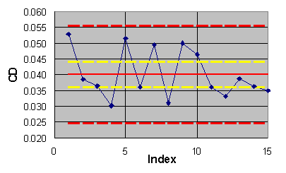
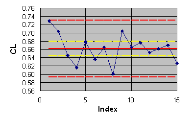
Figure 6.1 ECARP pseudo-time series for lift coefficient.
Figure 6.2 ECARP pseudo-time series for drag coefficient.
For the data of Table 6.1, the lift and drag outcomes do seem to be
drawn from the same (collective) computational process. Hence, we must
declare the computed lift to be 0.662 with a standard uncertainty of ![]() and the computed drag to be 0.0401 with a standard uncertainty of
and the computed drag to be 0.0401 with a standard uncertainty of ![]() .
For reporting purposes, usual practice is to multiply the standard uncertainty
by a coverage factor of two which would give a confidence level of 95%
for a normal distribution. The confidence intervals at 95% confidence for
the means are shown in figures 6.1 and 6.2 by dashed yellow lines. The
confidence intervals at 95% confidence to be used for each replication
are
.
For reporting purposes, usual practice is to multiply the standard uncertainty
by a coverage factor of two which would give a confidence level of 95%
for a normal distribution. The confidence intervals at 95% confidence for
the means are shown in figures 6.1 and 6.2 by dashed yellow lines. The
confidence intervals at 95% confidence to be used for each replication
are ![]() for the lift coefficient
and
for the lift coefficient
and ![]() for the drag coefficient.
In essence, we expect to find future outcomes lying between the dashed
red lines.
for the drag coefficient.
In essence, we expect to find future outcomes lying between the dashed
red lines.
6.3 Application to ECARP results divided into two groups
The scatter and means for both coefficients seems to be smaller for
the outcomes obtained using two-equation turbulence models. We will check
whether such an observation is warranted statistically by dividing the
15 outcomes into two groups: (1) outcomes 1-9 and (2) outcomes 10-15 and
compare the resulting means and standard deviations using hypothesis testing.
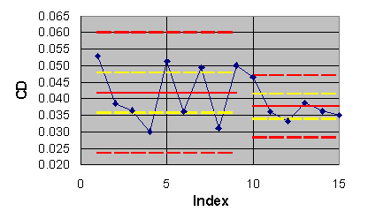
The population estimates are given in Table 6.2. The individual outcomes,
averages and limits (95% confidence) are shown in Figures 6.3 and 6.4 with
blue diamonds, solid red lines and dashed red lines respectively.
|
|
|
|
|
|
||
|
|
|
|
|
|||
|
|
|
|
|
|
|
|
|
|
|
|
|
|
|
|
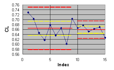 Table 6.2
Division of ECARP results for hypothesis testing.
Figure 6.3 ECARP lift coefficient results divided into two groups.
A crude test of the statistical significance of the difference in the means is given by comparison of the confidence intervals for the means (yellow dashed lines). If the intervals overlap, the null hypothesis is satisfied, although not exactly at the confidence level used to compute the intervals. The confidence intervals of the means in both Figures 6.1 and 6.2 overlap. Hence, we must declare, for this crude test, that our observations do not indicate that the means from the two types of solution methods are different.
 Figure
6.4 ECARP drag coefficient results divided into two groups.
Standard hypothesis tests using the t and F statistics provide a more refined comparison at a chosen level of confidence7, albeit at the expense of having to assume that the observations are normally distributed. We will carry out the tests for the lift coefficient first. We begin by checking the null hypothesis for the population standard deviations. The F statistic for the observations is
![]()
From a table of the percentage points of the F distribution, we compute the following values for 95% confidence with nine observations for the first group of computations and six for the second:

We reject the null hypothesis if ![]() is greater than the first F value or less than the second F value. Since
neither criterion is satisfied, we must declare that our observations do
not indicate that the lift coefficient standard deviations from the two
types of solution methods are different.
is greater than the first F value or less than the second F value. Since
neither criterion is satisfied, we must declare that our observations do
not indicate that the lift coefficient standard deviations from the two
types of solution methods are different.
Because the null hypothesis for the standard deviations is not rejected, the next step is to pool the standard deviations for the two groups, weighting them by their degrees of freedom:
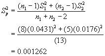
or
![]()
The t statistic is computed as follows:
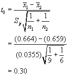
The criterion for rejecting the null hypothesis is
![]()
Comparing the two values shows that the criterion is not satisfied. Hence, we must declare that our observations do not indicate that the lift coefficient means from the two types of solution methods are different.
We carry out the tests for the drag coefficient next. The F-statistic for the observations is
![]()
The percentage points of the F distribution do not change from the lift case. Since neither criterion is satisfied, we must declare that our observations do not indicate that the drag coefficient standard deviations from the two types of solution methods are different.
Computing the pooled standard deviation gives:
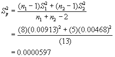
or
![]()
The t statistic is:
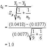
The percentage points of the t distribution do not change for the drag case. Comparing the two values shows that the criterion for rejection of the null hypothesis is not satisfied. Hence, we must declare that our observations do not indicate that the drag coefficient means from the two types of solution methods are different.
We will apply the above method of analysis to selected outcomes from
the collective computational process of this workshop in Section 8.