DPW-7 Data Submittal Forms and Postprocessing Information
Data Submissions, Errata, and Clarifications
DPW-7 is collecting data using a Tecplot-readable format with that template data
forms provided below. Please complete as much of each form as possible, including
the auxiliary data at the top of each form identifying the dataset. Forms are
provided for solver metrics, force/moment data, side-of-body separation data,
trailing edge separation data, and sectional cut data. Additionally, standard
views of contours of the solutions are requested.
Tecplot macros are provided
that will automatically extract data on the surface at the required cut
locations (see below for more details of cut locations), and generate contour
plots and streamlines with specific views.
Tecplot has graciously agreed that all participants who do not have access to
Tecplot may request a free extended evaluation license of 360 for use in
the AIAA Drag Prediction Workshop. If you are interested, please
email dpwaiaa@gmail.com.
Please email Tecplot-readable Data Submittal Forms to DPW-7 at
dpwaiaa@gmail.com.
Tecplot Macro Scripts
Tecplot Macro Scripts are provided for extracting wing section cuts and standard contour plots (Requires Tecplot 2019 Release 1 or newer):
- DPW-VII.SectionalCutter_v7c.mcr - wing section pressure cuts
- DPW-VII.Images_v7.mcr - contour plots and streamlines
Data Forms
For Cases 1-6, please submit a single set of forms for a common solution family
based on the same solver, turbulence model, grid type, etc.
A separate set of forms should be submitted for each solver, turbulence model,
grid type, etc.
Case 4 results can be included in the forms that also apply to the most similar
grid type. Otherwise Case 4 results can be given in a separate set of forms.
Case 1 - CRM Wing-Body Grid Convergence Study:
Case 1a. Re = 20M (Required)
Case 1b. Re = 5 M (Optional)
- DPW-VII.DataForm_Case1_GridMetrics_v7.dat - grid metrics for grid convergence studies
- DPW-VII.DataForm_ForceMoment_v7.dat - forces and moments (total, pressure skin friction, wing, fuselage) for Cases 1-6
- DPW-VII.DataForm_Sectional_Lift_and_Moment_Alpha_v7.dat - sectional lift and moment at each section vs. angle of attack for Cases 1-6
- DPW-VII.DataForm_Sectional_Lift_and_Moment_Span_v7.dat - sectional lift and moment at each section vs. span for Cases 1-6
- DPW-VII.DataForm_SectionalCuts_v7.dat - sectional pressure and skin friction coefficients for Cases 1-6
- DPW-VII.DataForm_TE_Separation_v7.dat - trailing edge separation location for Cases 1-6
- DPW-VII.DataForm_SOB_Separation_v7.dat - side-of-body separation location for Cases 1-6
Please update the GridID variable (DATASETAUXDATA GridId = "???") in
the templates from "CommonMB", "CommonOverset", etc.
using the nomenclature from the DPW7 provided grids website:
https://dpw.larc.nasa.gov/DPW7
Please update the TurbulenceModel variable (DATASETAUXDATA TurbulenceModel = "???") in the template using the common
turbulence model nomenclature from the Turbulence Modeling Resource web site:
https://turbmodels.larc.nasa.gov
Case 2 - CRM Wing-Body Alpha Sweep:
Case 2a. Re = 20M (Required)
Case 2b. Re = 5M (Optional)
Please append Case 2 data to above files with Case 1 data
- DPW-VII.DataForm_ForceMoment_v7.dat
- DPW-VII.DataForm_Sectional_Lift_and_Moment_Alpha_v7.dat
- DPW-VII.DataForm_Sectional_Lift_and_Moment_Span_v7.dat
- DPW-VII.DataForm_SectionalCuts_v7.dat
- DPW-VII.DataForm_TE_Separation_v7.dat
- DPW-VII.DataForm_SOB_Separation_v7.dat
Case 3 - CRM Wing-Body Reynolds Number Sweep At Constant CL (Required)
Please append Case 3 data to above files with Case 1-2 data
Case 4 - CRM Wing-Body Grid Adaptation -Alpha Sweep [Optional]:
Please append Case 4 data to above files with Case 1-3 data
Case 5 - Beyond RANS [Optional]:
Please append Case 5 data to above files with Case 1-4 data
Case 6 - CRM WB Coupled Aero-Structural Simulation [Optional]:
Please append Case 6 data to above files with Case 1-5 data.
Please also complete the Bending and Twist Data Form.
- DPW-VII.DataForm_ForceMoment_v7.dat
- DPW-VII.DataForm_Sectional_Lift_and_Moment_Alpha_v7.dat
- DPW-VII.DataForm_Sectional_Lift_and_Moment_Span_v7.dat
- DPW-VII.DataForm_SectionalCuts_v7.dat
- DPW-VII.DataForm_TE_Separation_v7.dat
- DPW-VII.DataForm_SOB_Separation_v7.dat
- DPW-VII.DataForm_Case6_BendingTwist_v7.dat - calculated section twist and bending from Case 6 Coupled aero-structural simulation
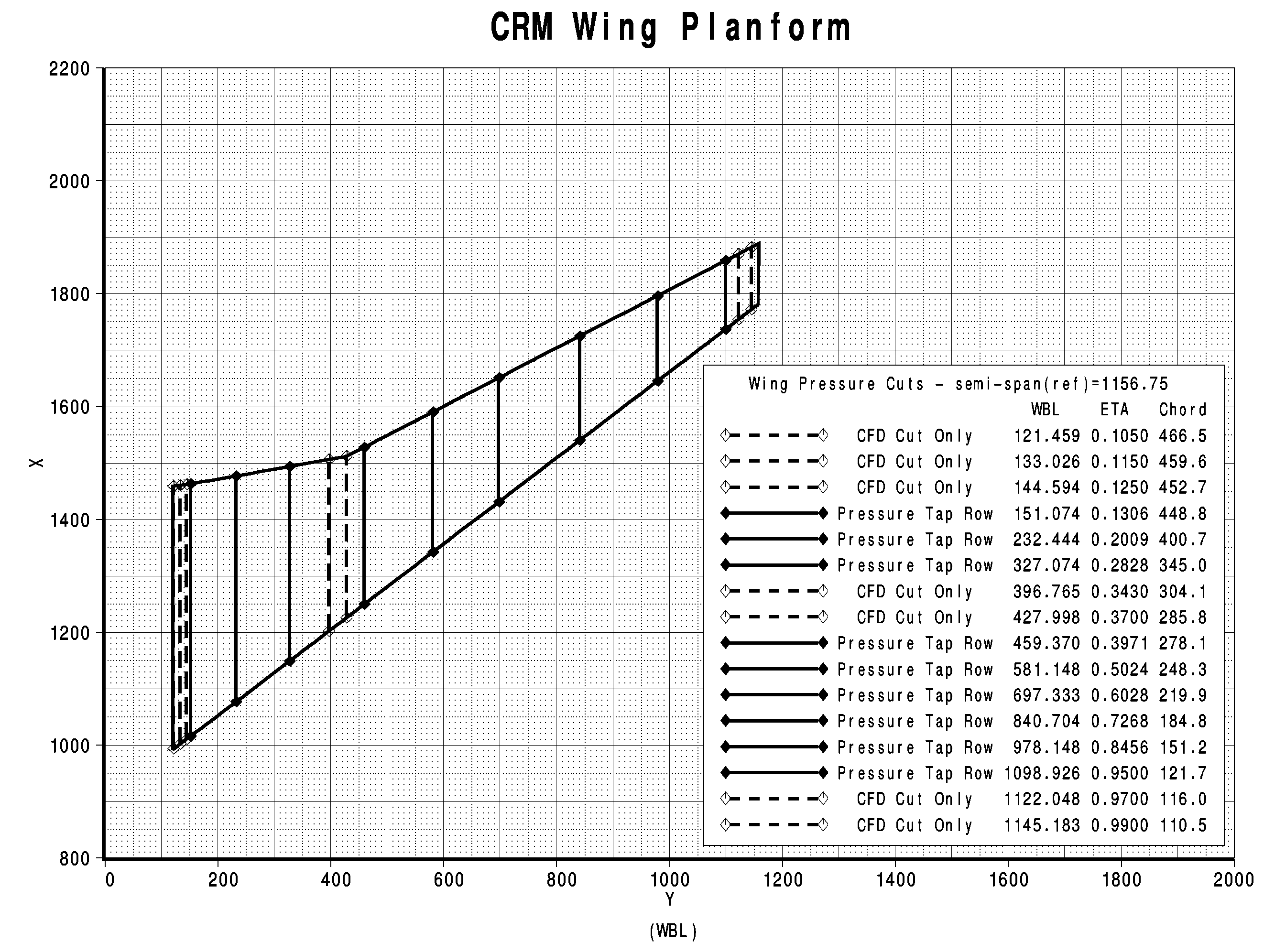
Wing Section Cut Locations
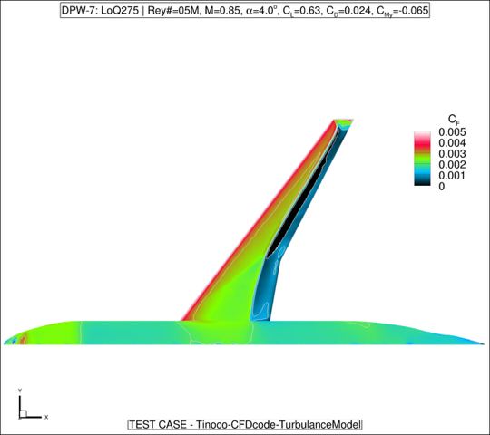
Pressure Coefficient (Cp) and Skin Friction Coefficient (Cf) Contours and Surface Streamlines
A major set of desired inputs from the CFD are computed surface streamlines for
comparison between CFD codes. This is particularly important for ascertaining
the agreement/disagreement with regions of separation and other flow features
of interest. Below are examples of surface streamline plots with contours of
surface coefficient of pressure and skin friction coefficient.
Please see the section below for details about the committee provided Tecplot macro file
for image generation to reduce work load and increase consistency across the participants.
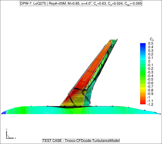
View 1: Top view of fuselage/wing with Cp contours and streamlines (above)
and Cf contours (below)
Note that values listed in the header are made-up
In all cases for unsteady methods, mean streamlines and skin friction
contours should be plotted.
In the pressure coefficient contour, the Tecplot color map "Small Rainbow".
It is given by:
| LEVEL | R | G | B |
| 0.00 | 0 | 0 | 255 |
| 0.25 | 0 | 255 | 255 |
| 0.50 | 0 | 255 | 0 |
| 0.75 | 255 | 255 | 0 |
| 1.00 | 255 | 0 | 0 |
with a recommended range (shown in the figure) of -1.20 to 0.50, with steps of 0.10.
In the skin friction contours, the Tecplot color map is provided as cfmap_tecplot.map
(https://hiliftpw.larc.nasa.gov/Workshop4/cfmap_tecplot.map).
It is given by:
| LEVEL | R | G | B |
| 0.00 | 0 | 0 | 255 |
| 0.25 | 0 | 191 | 255 |
| 0.50 | 127 | 255 | 0 |
| 0.75 | 255 | 0 | 64 |
| 1.00 | 255 | 255 | 255 |
with a recommended range (shown in the figure) of 0 to 0.005, with steps
of 0.001. When plotting CFx, the recommended range is -0.002 to 0.005 with
steps of 0.001.
The "lighting" has been turned off; which reduces the 3-dimensional
appearance of the objects, but it improves the interpretability of the colors.
If everyone removes lighting and follows the color scheme and range detailed
here, then the resulting CFD plots should be reasonably easy to compare
directly with one another.
For direct CFD comparisons with other CFD, some recommended views
(including Tecplot nomenclature for orientation) are shown below, where
the configuration is in full-scale inches with the forward most point
on the fuselage at (92.5,0.0,198.0). Note that the axes are assumed to have
the X-axis running from fuselage nose to tail, Y-axis running from symmetry
plane to wing tip, and Z-axis running from fuselage keel to crown.
In Tecplot, the "use perspective" feature is not turned on for any views.
NOTE: Eight views are shown. Please provide as many as you are able.
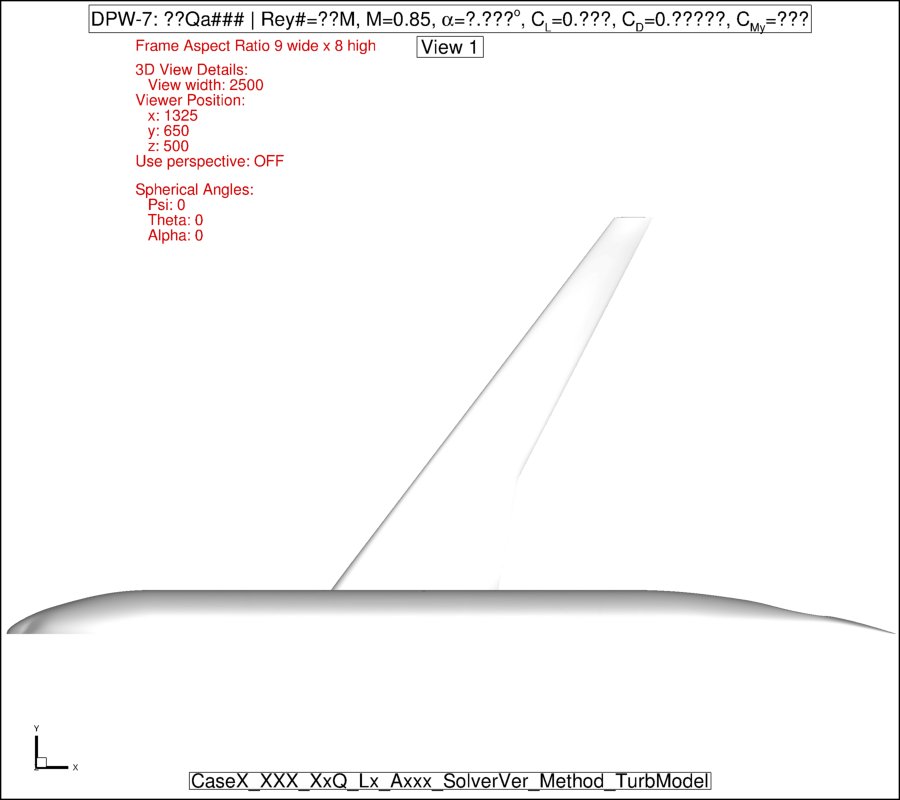
View 1: Top view of fuselage/wing
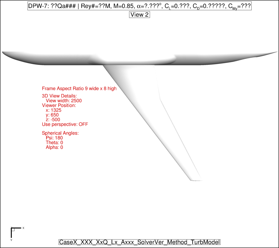
View 2: Bottom view of fuselage/wing
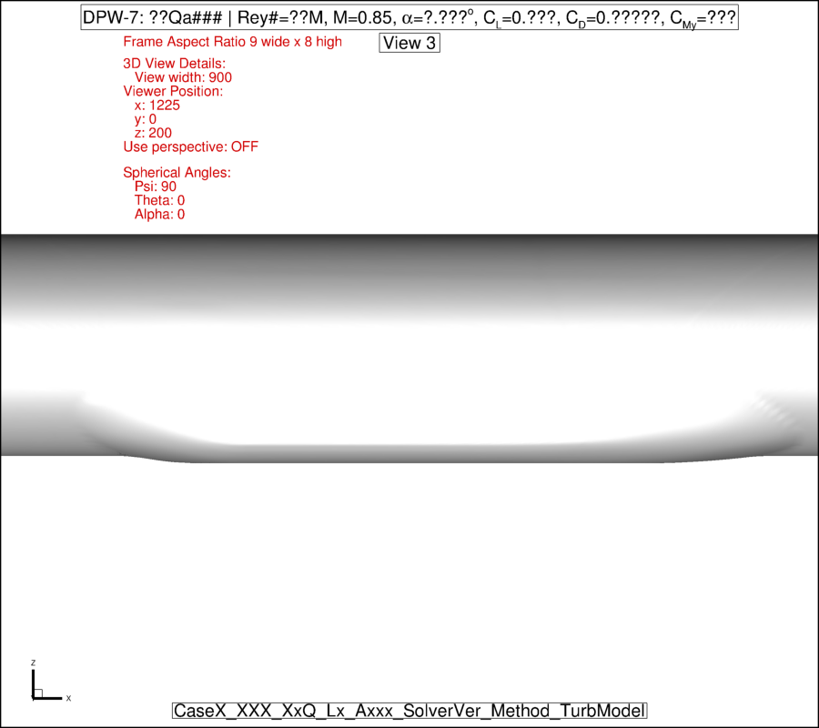
View 3: Fuselage side-of-body (remove wing from view)
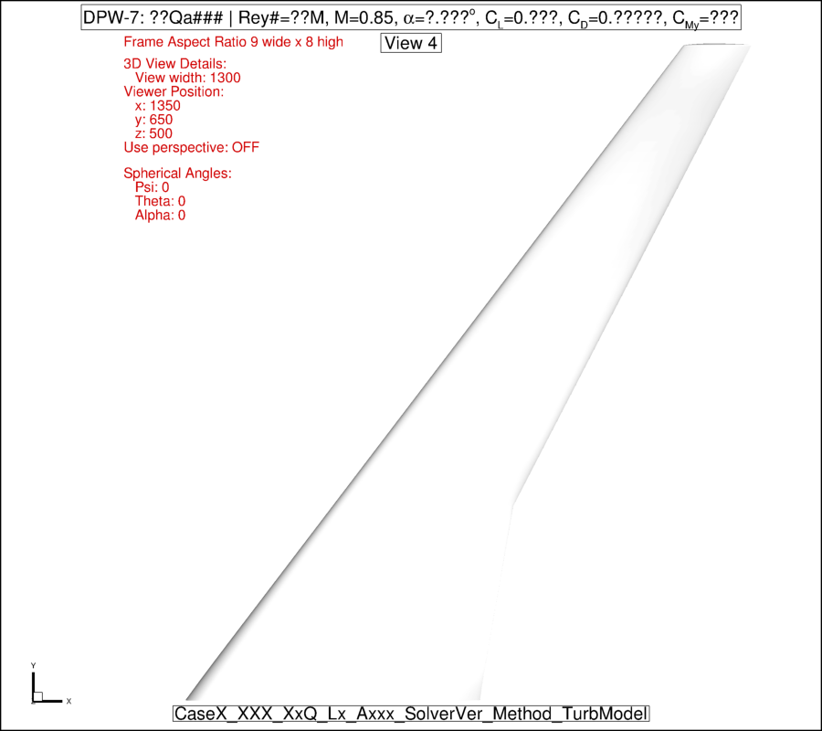
View 4: Top view of wing (remove fuselage from view)
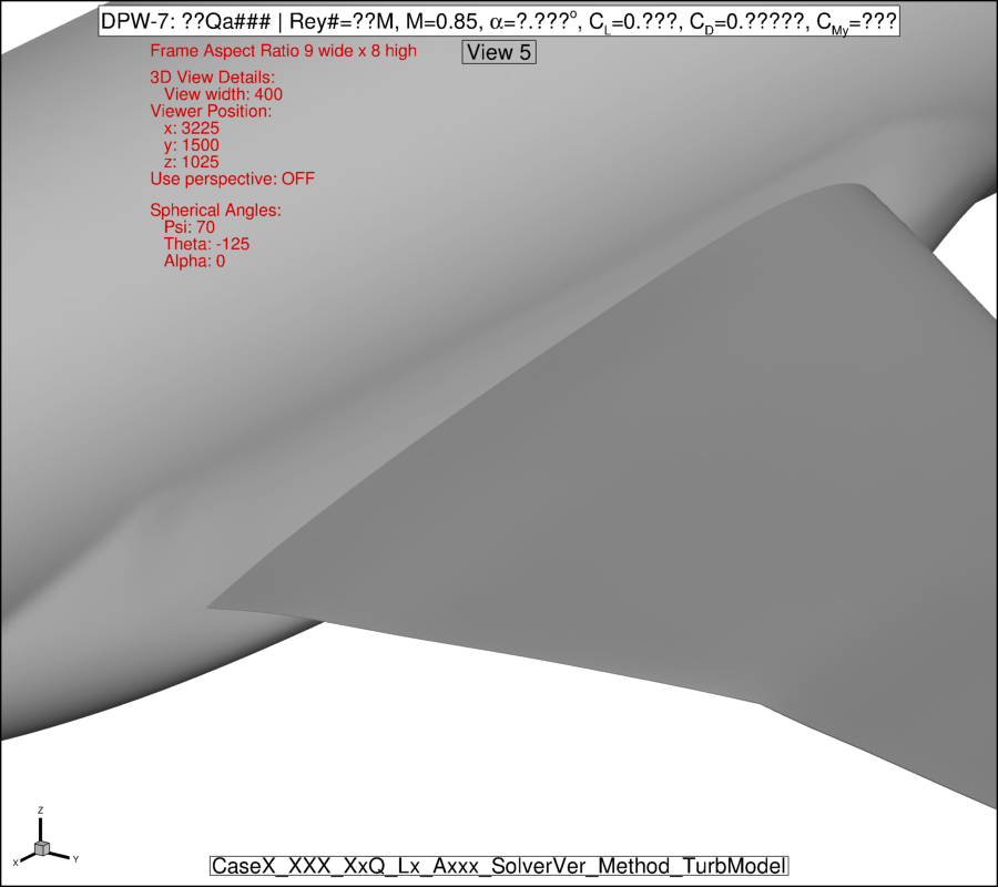
View 5: View of side-of-body near trailing edge of wing
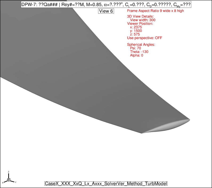
View 6: View of wing-tip region of wing
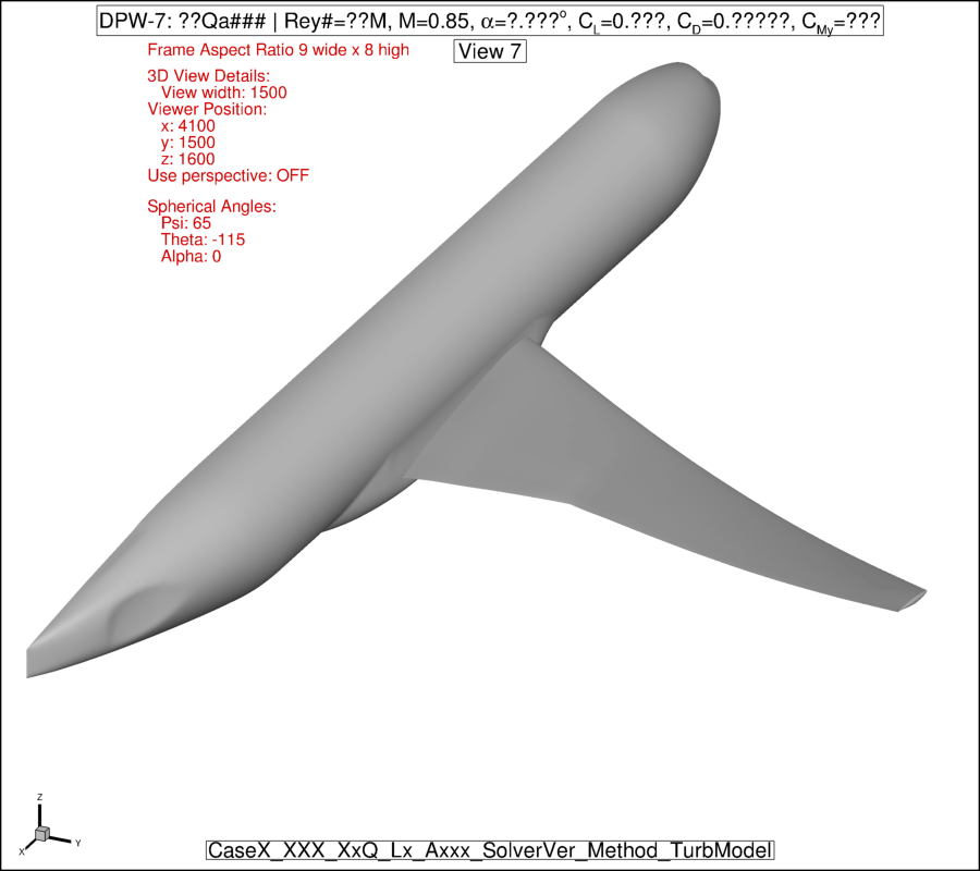
View 7: Isometric view of fuselage/wing from the back
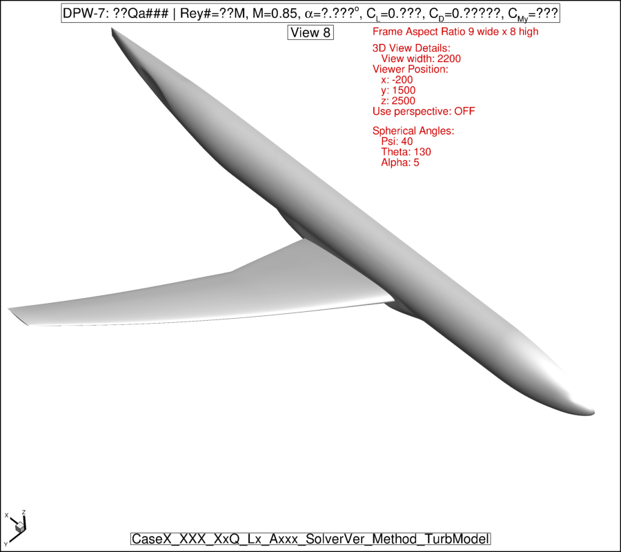
View 8: Isometric view of fuselage/wing from the front
Committee provided Tecplot macro file for image generation
A Tecplot macro has been provided to generate all of the prescribed views of
a loaded solution, define the prescribed color maps and levels for contours,
and automatically generate streamtraces in the regions of interest.
The macro is intended to be run after a dataset has been read into Tecplot.
The user should either load their dataset manually and then run the macro
(Scripting --> Run Macro) or customize the macro file with the addition of a
$!ReadDataSet
acro command appropriate for your dataset.
If the $!ReadDataSet
command has been added, the macro file can be run in batch mode at a
terminal command prompt like this:
tec360 <-mesa> -b -p DPW-VII.Images_v4.mcr
The user is also required to populate some variables to define the case and condition:
# CaseX - Case [Case1/Case2/Case3/Case4/Case5/Case6]
# XXX - First-author participant's last name (or organization)
# XxQ - Condition Q [LoQ/HiQ/NoQ]
# RxxM - Reynolds Number [05/20/30]
# Lx - Grid Level [L1/L2/L3/L4/L5/L6]
# Axxx - Angle of Attack [275/300/325/350/375/400/425]
# (use C058 for Fixed CL=0.58 case)
#
# Grid/SolverVer/Method/TurbModel should be descriptive labels specific to your case
#
# Label for this solution
$!VarSet |SolutionLabel| = 'CaseX_XXX_XxQ_RxxM_Lx_Axxx_Grid_SolverVer_Method_TurbModel'
$!VarSet |OutputDirectoryPath| = '' # Images will be saved to this path
# NOTE: Use '' if Tecplot run from within desired directory
$!VarSet |Q| = '??Qa???' # Aeroelastic shape [ie LoQa275/HiQa275]
$!VarSet |REYN| = '??' # Reynolds number [05 or 20 or 30] in millions (based on reference chord)
$!VarSet |MACH| = '0.85' # Mach number
$!VarSet |ALPHA| = '0.???' # Angle-of-Attack
$!VarSet |CL| = '0.???' # Lift Coefficient
$!VarSet |CD| = '0.?????' # Drag Coefficient
$!VarSet |CMy| = '???' # Pitching Moment Coefficient
The user must provide information identifying the variable number corresponding to the (X, Y, Z) coordinates, Cp, Cf, Cfx, and (U, V, W) velocity vector (or CF vector) for use in streamtraces:
$!VarSet |Xvar| = 1 # Variable number of X coordinate
$!VarSet |Yvar| = 2 # Variable number of Y coordinate
$!VarSet |Zvar| = 3 # Variable number of Z coordinate
$!VarSet |CPvar| = 4 # Variable number of Cp contours
$!VarSet |CFvar| = 8 # Variable number of Cf contours
$!VarSet |CFXvar| = 5 # Variable number of Cfx contours
$!VarSet |Uvar| = 5 # Variable number of streamtrace vector x-component (u-velocity)
$!VarSet |Vvar| = 6 # Variable number of streamtrace vector y-component (v-velocity)
$!VarSet |Wvar| = 7 # Variable number of streamtrace vector z-component (w-velocity)
The user must define the fieldmaps that define the fuselage/body surface and the fieldmaps that define the wing surface:
$!VarSet |BodyMaps| = '1' # Fieldmaps of the body/fuselage dataset ('1-2','1,3,5-6',etc.)
$!VarSet |WingMaps| = '2' # Fieldmaps of the wing dataset ('1-2','1,3,5-6',etc.)
Optionally, the macro will attempt to identify the correct Zones for the Body & Wing components based on the maximum Y_coordinate value of each Zone if the user leaves the inputs as:
$!VarSet |BodyMaps| = '' # Fieldmaps of the body/fuselage dataset ('1-2','1,3,5-6',etc.)
$!VarSet |WingMaps| = '' # Fieldmaps of the wing dataset ('1-2','1,3,5-6',etc.)
Note that the coordinate axes are assumed to have the X-axis running from fuselage
nose to tail, Y-axis running from symmetry plane to wing tip, and Z-axis running
from fuselage keel to crown. If the coordinates of your dataset need to be reversed,
that can be accomplished by setting |Xrev|,|Yrev|,|Zrev| variables to 1 (from their
default value of 0).
The coordinates of the input data will be scaled and translated automatically to
align with a configuration in full-scale inches with the forward most point on
the fuselage at (92.5,0.0,198.0).
Finally, the user may also need to define the Solution Time that should be active
for the exported images. If the macro produces blank images with only titles and
legends and your data set includes data for more than one time step, you may need
to identify a specific time to be used to make the plot. Look for the slider bar
in the Plot sidebar and identify the Solution Time to be used.
$!VarSet |PlotTime| = '' # Tecplot SolutionTime to export for time-accurate data sets
# NOTE: Leave |PlotTime| = '' if no solution time needs to be set
After the above customization and labelling has been completed, the user can run the macro, which will generate the requested images corresponding to the views above.